
- Home
- Getting Started
- Documentation
- Release Notes
- Tour the Interface
- Tour the Layers
- JMARS Video Tutorials
- Lat/Lon Grid Layer
- Map Scalebar
- Nomenclature
- Crater Counting
- 3D
- Shape Layer
- Mosaics
- Map
- Advanced/Custom Maps
- Graphic/Numeric Maps
- Custom Map Sharing
- Stamp
- THEMIS
- MOC
- Viking
- CRISM Stamp Layer
- CTX
- HiRise
- HiRISE Anaglyph
- HiRISE DTM
- HRSC
- OMEGA
- Region of Interest
- TES
- THEMIS Planning
- Investigate Layer
- Landing Site Layer
- Tutorials
- Video Tutorials
- Displaying the Main View in 3D
- Finding THEMIS Observation Opportunities
- Submitting a THEMIS Region of Interest
- Loading a Custom Map
- Viewing TES Data in JMARS
- Using the Shape Layer
- Shape Layer: Intersect, Merge, and Subtract polygons from each other
- Shape Layer: Ellipse Drawing
- Shape Layer: Selecting a non-default column for circle-radius
- Shape Layer: Selecting a non-default column for fill-color
- Shape Layer: Add a Map Sampling Column
- Shape Layer: Adding a new color column based on the values of a radius column
- Shape Layer: Using Expressions
- Using JMARS for MSIP
- Introduction to SHARAD Radargrams
- Creating Numeric Maps
- Proxy/Firewall
- JMARS Shortcut Keys
- JMARS Data Submission
- FAQ
- Open Source
- References
- Social Media
- Podcasts/Demos
- Download JMARS
Viewing TES Data in JMARS
The purpose of this tutorial is to walk users through the process of opening JMARS, navigating to the MER-B (Opportunity) landing site at Meridiani Planum, opening the TES Layer and using the TES Layer to view spectral data in JMARS. The TES Layer is currently only available in the THEMIS Team Release of JMARS, which will be used for this tutorial.
Step 1: Opening JMARS and Navigating to Meridiani Planum
- Double-click the JMARS icon on your desktop
- Enter your JMARS user name and password. If you do not have a user name and password, follow the instruction under the appropriate "Getting Started" link on the Main Page.
- At this point, the Layer Manager should only have the MOLA Shaded Relief Layer and the Lat/Lon Layer loaded.
- In the Lon/Lat box in the upper-left corner of the Viewing Window, enter the coordinates "-5.94E, -1.98"
- The Main View should now be centered over Meridiani Planum.
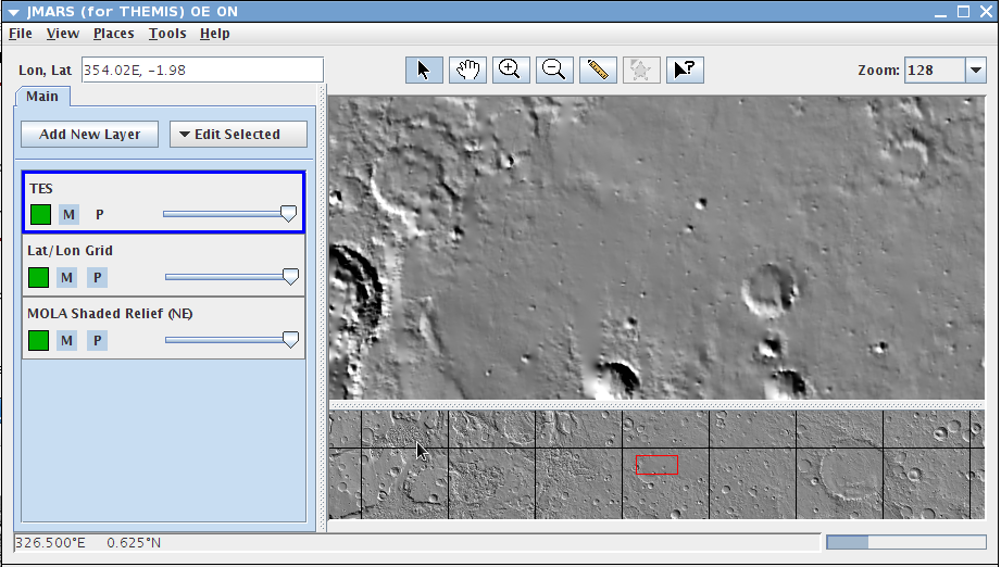
Step 2: Opening the TES Layer
- Using the "Zoom" menu in the top-right corner of the Viewing Window, zoom the Main View to 256 ppd.
- Left-click in the Panner View, select "Zoom" and select "128 Pix/Deg".
- The TES Layer requires a large amount of data to be loaded from the TES Database. The less area displayed in the Main and Panner Views the faster the layer will refresh when changes are made. Depending on your computer and internet connection, this refresh time may still be large.
- In the Layer Manager, click "Add New Layer" -> "Spectra" -> "TES", then double-click on the "TES" layer to access the focus panel.
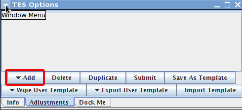
- The focus panel should be blank except for the buttons at the bottom.
Step 3: Viewing TES Hematite Concentration Data
- Click "Add" at the bottom of the TES focus panel --> then click "Blank Template" to create a new TES context.
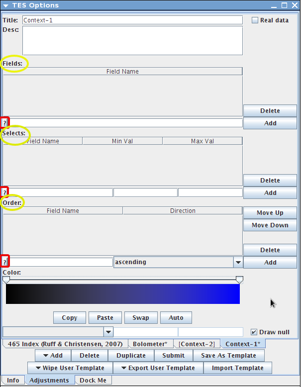
- The focus panel will fill with a number of fields for loading, sorting and colorizing TES data.
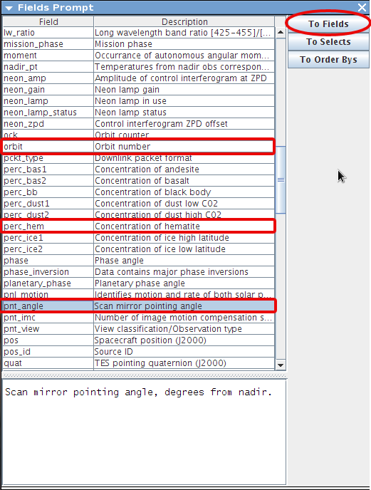
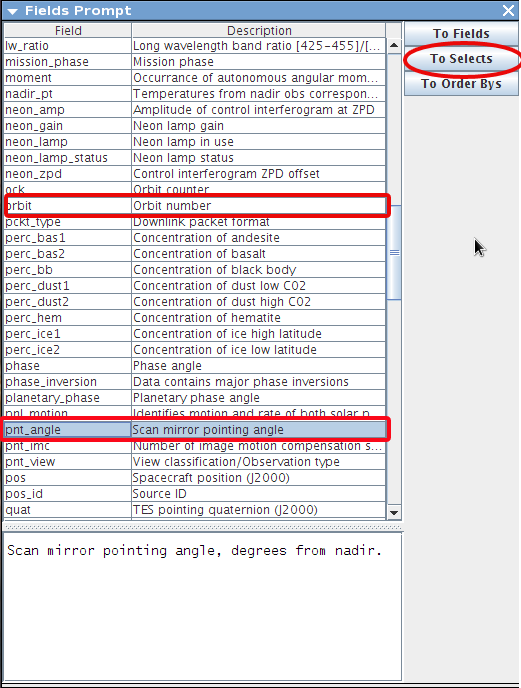
- Click on the "?" button to the left of the first input line to view a list of all available TES database fields. This is located under "Fields".
- Load Database Fields into the TES Layer, This is under "Selects":
- Click on the "?" under "Selects" --> In the list of database fields, highlight "orbit" and click the "To Fields" button.
- In the "Fields" section of the focus panel, "orbit" will appear in the input box. Click "Add" to load it into the TES Layer. (The "orbit" will move from the input box into the list of loaded fields.)
- Repeat this process for the "pnt_angle" (TES pointing mirror angle), "perc_hem" (Hematite concentration) and "emissivity" fields.
- Select Filtering Values for the Loaded Database Fields
- In the list of database fields, highlight "orbit" and click the "To Selects" button.
- In the "Selects" section of the focus panel, "orbit" will appear in the first input box. The second and third input boxes are the minimum and maximum allowable values, respectively. Enter a minimum value of "0" and a maximum value of "10000".
- Repeat this process for "pnt_angle" with a minimum of "0" and a maximum of "5". This will ensure that only nadir-pointing observations are displayed.
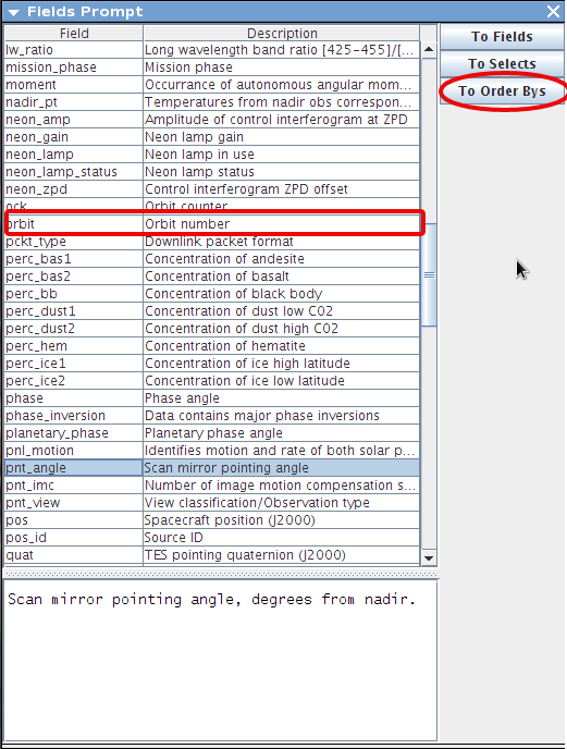
- Specify Ordering Parameters
- First click the "?" under "Order"
- In the list of database fields, highlight "orbit" and click the "To Order Bys" button.
- In the "Order" section of the focus panel, "orbit" will appear in the input box. Select "Ascending" from the drop-down menu and then click "Add".
- This will draw the TES observation footprints in the Viewing Window starting with the earliest observation.
- Specify Coloring Parameters
- In the "Color" section of the focus panel, you can select a color pattern.
- Right-click on the right-hand slider on the color bar, then select "Built-in Color" -> "Inverted Spectrum"
- The two input boxes represent the minimum and maximum values of the given color spectrum. Enter "-0.5" for the minimum and "0.5" for the maximum.
- Values higher than the maximum value will be colorized as if they were the maximum value. Values lower than the minimum values will be colorized as if they were the minimum value.
- Although a negative percent composition is not possible, the "-0.5" value is used to make the coloring more intuitive in this case. (The low concentrations will be displayed as cooler hues and the higher concentrations will be displayed as warmer hues.)
- Un-check the "Draw Null" checkbox at the bottom-right corner of the focus panel.
- This will prevent TES footprints without "perc_hem" data from being drawn in the Viewing Window.
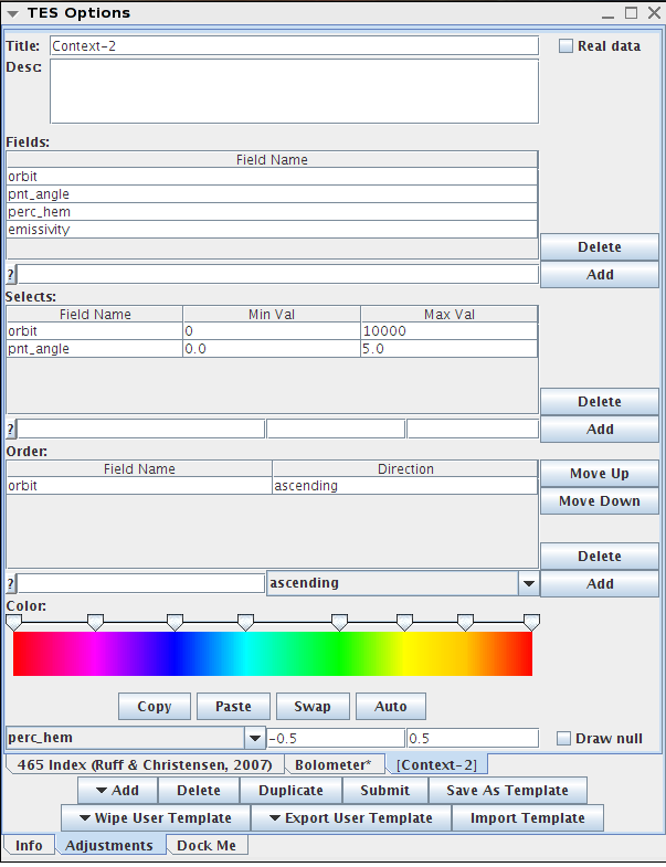
- Click on the "Submit" button at the bottom of the focus panel to request the specified information from the TES Database.
- Before submitting the request, the focus panel should look like the first example below.
- Depending on your computer and internet connection, it may take the TES Layer a few minutes to refresh.
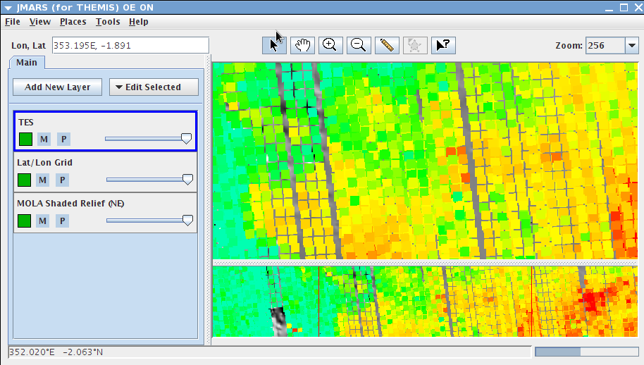
- After the request data has been loaded, the Viewing Window should look like the second example below.
Step 4: Viewing Actual TES Data Values
- To see the TES detector footprints more clearly, zoom the Main View to 512 ppd.
- In the "Selects" section of the TES Layer focus panel, highlight the "orbit" row and click the "Delete" button to the right.
- Add a new search constraint using the three input boxes at the bottom of the "Selects" section. In the first box, type "orbit", the second type "5500" and in the third type "6000".
- Click "Submit" at the bottom of the focus panel to submit the new data request.
- After the TES Layer has refreshed, it is much easier to see the individual TES detector footprints.
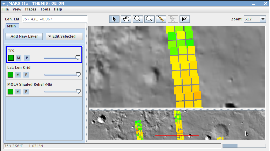
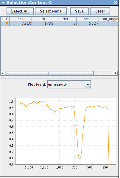
- To view the data associated with one of the footprints, left-click on it. This will bring up a data display window.
- If multiple footprints overlap the point you clicked on, multiple rows will appear in the data display window.
- The data table displays values for all of the loaded fields (listed in the "Fields section of the focus panel) which have single-value data. (ie: mirror pointing angle, surface temperature, etc)
- Note that emissivity is not included in the table because it is not a single-value data field.
- To graph the emissivity in the plotting field at the bottom of the window, select "emissivity" from the drop-down menu. Then click on one of the rows in the data table. The emissivity graph for that particular footprint will then appear in the plotting field.
Congratulations! You have finished the sixth JMARS tutorial!
PREVIOUS: Loading a Custom Map NEXT: Using the Shape Layer